


The transmission of monetary policy: from mortgage rates to consumption
Published as part of the ECB Economic Bulletin, Issue 4/2025.
1 Introduction
Monetary policy affects consumption via multiple channels, with different effects on households’ decisions. By preserving price stability, monetary policy supports consumption in the medium run, as it protects the purchasing power of households. In the short run, however, tighter monetary policy typically dampens private consumption.[1] First, higher interest rates reduce current consumption, as they increase the attractiveness of savings via the “intertemporal substitution channel”. Consumption decisions also respond to changes in policy rates as they affect the prices of financial and real assets and generate wealth effects (the balance sheet channel of monetary policy). In parallel, interest rate changes affect the real economy and the evolving labour market conditions, thereby changing income prospects, with consequences for households’ consumption decisions. Monetary policy also affects household finances via its impact on cash flows from household debts and assets. Higher interest rates raise interest payments by indebted households, reducing the cash flow available for spending, while increasing the interest revenues on interest-bearing assets, raising the cash flow for asset holders. Given these two counteracting forces, the size and sign of the overall cash flow effects for any individual household depend on their net interest rate position.[2] This mechanism is referred to as the cash flow channel of monetary policy.
Following policy rate hikes, the cash flow channel of monetary policy may pose persistent headwinds to consumption. This article analyses the impact of monetary policy decisions via changes in debt servicing costs and particularly mortgage payments, while abstracting from other direct channels and general equilibrium effects.[3] This focus is dictated by the relevance of mortgages for euro area households, as one in four households has a mortgage, as well as by the heterogeneity of the euro area mortgage market across countries and income groups. To this end, we present new evidence using household-level information on the timing of changes in mortgage payments and consumption from the ECB’s Consumer Expectations Survey (CES). In particular, we show that due to (i) the higher prevalence of fixed-rate mortgages (FRMs) compared with the past, and (ii) the smaller gap between interest rates on outstanding amounts and interest rates on new loans compared with the start of previous monetary policy tightening cycles, the impact on consumption through the mortgage channel is likely to be more protracted in the 2022-23 monetary policy tightening cycle. We aim to quantify this specific effect. Other factors may act in the opposite direction, such as positive developments in real incomes due to the recovery from the recent crises, and the possible reductions of high savings, which were to some extent driven by uncertainty or income misperceptions.[4] The rest of this article will abstract from these other channels and focus exclusively on quantifying the delayed tightening effects through the cash flow channel via mortgages.
2 Characterising the euro area mortgage market
Differences in the structure of mortgage contracts across countries shape the timing of the effects. During the 2022-23 tightening period, interest payments on adjustable-rate mortgages (ARMs) reacted quickly. However, for many households the increase in mortgage payments is still to come, as their temporarily fixed rates (e.g. for five or ten years) expire and are repriced at new market rates. The new rates are likely to be higher since many of these loans were contracted in a period of lower mortgage rates. In the euro area, about one-quarter of mortgages are pure ARMs, while a little over one-third have rates that are fixed for longer than ten years. The remaining mortgages are fixed for several years and are then set to be repriced (Chart 1). The distribution of these fixation periods means there will be a staggered series of mortgage rate repricings in the coming years, leading to higher interest rates. In total, about 10% of all loans currently have fixed interest rates that will be adjusted in the next three years, while 20% will be repriced by 2030.[5] These patterns differ across countries. Among the largest euro area economies, ARMs are traditionally more prevalent in Spain and, to a lesser extent, Italy, while at least some level of interest rate fixation is more common in Germany and France. In a nutshell, the prevailing loan structure implies that the effect of interest rate changes on mortgage payments is subject to considerable lag.
Chart 1
Remaining interest rate fixation period by country
(percentages of mortgagors)

Sources: ECB (CES) and ECB calculations.
Notes: The statistics are computed from the CES housing module administered in February 2025. “All” refers to all countries covered in the CES sample: Belgium, Germany, Ireland, Greece, Spain, France, Italy, Netherlands, Austria, Portugal and Finland. The shares are computed over respondents who have a mortgage outstanding and represent percentages of respondents rescaled by the annual survey population weights and individual loan outstanding balances. The latest data are for February 2025.
The timing of mortgage repricing also differs within countries, with shorter rate fixation periods more common for lower-income households. Lower-income households with a mortgage are more likely to have ARMs or FRMs with rate resets due in the next few years. Among the bottom 20% of the within-country income distribution, 32% of mortgages are ARMs, compared with 17% for the highest quintile (Chart 2, panel a). Additionally, among lower-income households, even mortgages set to reprice in more than three years have shorter average fixation than the same type of mortgages held by richer households. As a result, around 39% of all loans to lower-income households are set to reprice by 2030 compared with only around 20% for the highest income quintile (Chart 2, panel b). The share of mortgagors exposed to an increase in mortgage payments in the coming years is thus much higher among the poorest than the richest, as the distribution of mortgage types differs across incomes, even though the reduction in interest rates as from June 2024 will mitigate the impact. Financial constraints, information constraints and financial literacy may explain this. First, it is generally more expensive in the short term to choose an FRM when prevailing market rates are low. This leads poorer or more liquidity-constrained households to opt for contracts that are more attractive in the short term in periods of low interest rates, which are generally ARMs. Second, higher-income households have access to information and services that improve choices (e.g. access to loan brokers or other dedicated services). Finally, higher-income households tend to have higher levels of financial literacy.[6] This may explain why they are more likely to choose mortgages that are fixed for longer periods (during a low interest rate regime), despite the higher up-front cost which partly reflects the cost of hedging against interest rate risk when that risk is costly.
Chart 2
Remaining interest rate fixation period and share of repricing mortgages by income quintile
a) Fixation type | b) Mortgages repricing by 2030 |
|---|---|
(percentages of mortgagors) | (percentages) |
 |  |
Sources: ECB (CES) and ECB calculations.
Notes: The chart shows differences in mortgage fixation patterns across income groups, from Q1 (lowest income quintile) to Q5 (highest income quintile). Panel a) depicts the structure of fixation of mortgage loans for each income quintile – the quintiles are computed among all households in each country. The dashed blue section refers to fixed-rate loans that are set to be repriced within the next three years. The blue section corresponds to the share of FRMs with longer fixation horizons. Panel b) depicts the average share of loans repricing per year (percentage exposed to interest rate risk) across the projected years (2025-30) by income quintile. The latest data are for February 2025.
3 Tightening in the pipeline: simulating the evolution of average mortgage rates on outstanding balances
Since the ECB started cutting its policy rates, the average interest rate on the stock of mortgages has so far remained broadly flat despite the decline in rates on new loans. This is due to two distinct factors. First, the decline in market rates drove the rate on ARMs down, but mortgages with limited fixation periods are still repricing at higher rates than the ones at which they were issued. Second, loans that were issued at especially favourable lending conditions in the past are gradually being paid down, while new mortgages are issued at new conditions. In other words, the pass-through of the lending rate on new loans to the rate on the stock of loans will depend not only on lending rate developments, but also on loan dynamics and the joint distribution of residual maturities, residual fixation periods and average lending rates currently paid on the stock of loans. Given that mortgages have long maturities, this joint distribution will itself depend on the recent history of monetary policy cycles and lending dynamics. Standard time series models estimated over short samples are ill-suited to capture how these different factors play out.
Using detailed CES micro data, we developed a “micro-simulation” approach to project developments of household-level loan interest payments, which can then be aggregated. The micro-simulation approach allows us to simulate rates on the stock of mortgages consistent with the prevailing distribution of mortgages. This approach utilises the complete distribution of household-level loans, including outstanding amounts, interest rates paid, time until the next interest rate reset and maturity. We assume lending rates on new loans remain constant at their latest available level (dashed blue line in Chart 3, panel a). This allows us to abstract from further upward pressure on long-term interest rates that is currently priced in in forward curves. Next, we calculate the trajectory of the lending rate on each individual loan by adjusting the interest rate of existing loans with expiring fixation periods in the year they reprice (while doing so each year for ARMs) with the expected interest rate on new mortgages. Loans that are set to reach maturity by the end of any projection year are removed from the stock. Finally, we add new loans, randomly sampled from the survey, at the simulated rate for new loans, while assuming that lending growth also remains constant at its last observed level. We also calculate a risk premium by income quintile using mortgagors’ income information, calibrate it to the country-level risk premia, and apply it to the country-specific simulations for both new loans and repricing mortgages. The interest rates of adjustable, fixed and new mortgages are then aggregated and weighted by a combination of population weights and outstanding balances.
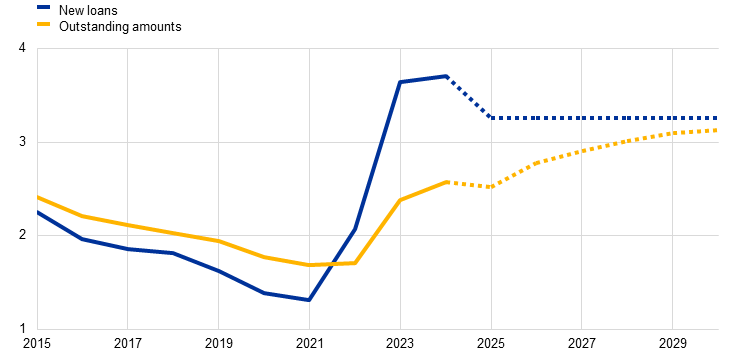
Chart 3
Lending rate simulations
a) Aggregate
(percentages per annum)
b) By income group
(percentages per annum)
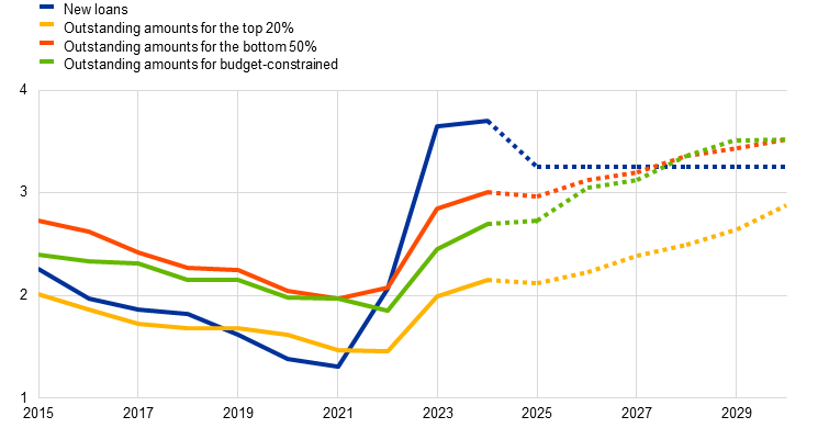
Sources: ECB (MIR, BSI, CES) and ECB calculations.
Notes: The chart depicts the interest rate paths for the rate on new loans (yearly average) and the outstanding amounts (end-of-year) of household mortgages. The micro-simulation (panel a: yellow line, panel b: yellow, red and green lines) takes into account the full set of available information at the individual level, and from 2025 to 2030 projects the rate on outstanding amounts using information on the remaining interest rate fixation period of mortgages at the individual level. For each projected year we calculate the interest rate based on the sampled stock of mortgages from February 2025, by adjusting the interest rate of the existing loans with expiring fixation periods in the year they expire, and the ARMs with the latest available country information for the rate on new mortgages. We calculate a risk premium by income quantile using household income information, apply it to the country-specific paths of the rate on new loans, and calibrate it to the macro country risk premia. To generate the backward-looking CES rate on outstanding amounts, we aggregate the reported interest rates on the stock of FRMs of all respondents from the year in which they were created. Budget-constrained households are defined as those with housing and food expenses above 75% of their total household income.
The latest data are for February 2025 for the CES mortgage stock and March 2025 for MIR and BSI.
Lending rates on the stock of loans are expected to continue increasing as long as they remain below the rates on new loans. The exercise shows that starting in mid-2025, lending rates on the stock of loans should increase (dashed yellow line in Chart 3, panel a) even when lending rates on new loans remain constant and the expected rise in long-term market rates is not incorporated. Intuitively, this should continue for as long as the rate on the stock of loans remains below the rate on new loans. Rates on outstanding amounts currently stand at around 2.4%. They are expected to converge towards the rate on new loans at a steady-state level of around 3.3%. The fact that the rate on the stock of loans is projected to continue increasing, despite the decline of the rate on new loans since its peak, stands in contrast to previous easing cycles and speaks to three factors: (1) a hiking cycle that started after a long period of low rates during which rates on the stock of loans had converged to low levels, (2) a less complete pass-through of rate hikes due to the higher share of fixed-rate mortgages and the pace and magnitude of the tightening cycle, and (3) the fact that the current interest rate cycle is expected to leave interest rates on new loans at higher levels than before 2021. In Box 1 we model the hypothetical effects of the current easing cycle had it occurred against the background of the lending rate configuration prevailing at the onset of the previous easing cycle, in October 2008.
Box 1
The state dependence of monetary policy: differences in pass-through across easing cycles
Unlike in previous easing cycles, lending rates on the stock of loans are expected to continue to rise despite the recent rate cuts. This is due to the fact that the pass-through of past policy rate changes to the stock of loans is still less complete than in the past. This can be seen in a simple summary statistic: the gap between the rate that households pay on their stock of loans and the one they would pay on any new loan.[7] This gap appeared historically elevated at the onset of the current easing cycle: it stood at 1.4 percentage points in May 2024, compared with 0.4 percentage points in October 2008 (Chart A). This is explained by the declining share of adjustable-rate mortgages (ARMs) and the specificities of the period around the latest tightening cycle, as detailed in the text of the article.
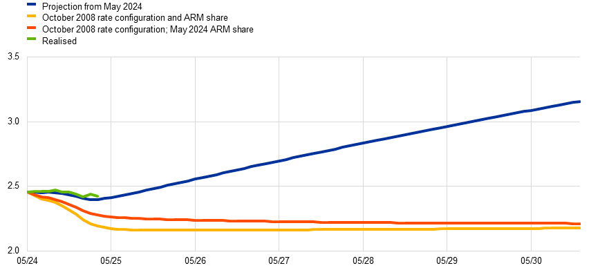
Chart A
Lending rate on new business and on outstanding amounts across easing cycles
(percentages per annum)

Sources: ECB (MIR) and ECB calculations.
Notes: Vertical lines are drawn in the month preceding the first rate cut of any easing cycle. The latest observation is for March 2025.
To assess how these effects dampen the impact of the rate cuts on mortgage payments and consumption, we run a counterfactual simulation of rates on outstanding amounts starting from the gap between rates on new business and outstanding amounts at the onset of the previous easing cycle (Chart B). To this end, we keep the same distribution of loans by residual maturities and fixation periods as in the latest Consumer Expectations Survey, but reset lending rates in each bucket to those that prevailed in October 2008: loans in the ARM bucket are set at the average lending rate on new business with short fixation in October 2008; fixed-rate loans are set at the rate on short or long-term fixation loans that prevailed when the loan was issued.[8] The same changes in lending rates on new loans and lending volumes as in the baseline simulation are then used to produce a counterfactual simulation of lending rates on outstanding amounts from October 2008, which is finally used to produce a counterfactual simulation from May 2024.
If the October 2008 rate configuration had prevailed in May 2024, the average rate would have declined faster up to mid-2025 and flattened thereafter, instead of resuming its increase (red line in Chart B). The lending rate on the stock of loans would have been around 0.6 percentage points lower as of the end of 2027, and as much as 1.1 percentage points lower by the end of 2030. Running the same counterfactual while also adjusting the share of ARM borrowers to the level seen in October 2008 (yellow line in Chart B) shows that the currently lower share of ARM borrowers explains less than 10% of the higher level of rates on outstanding amounts by the end of 2027. The fact that the rate on the stock of loans would have declined in the counterfactual simulation means that there would have been no further drag on consumption.
Chart B
Counterfactual changes in rates on outstanding amounts
(percentages per annum)
Sources: ECB (MIR, BSI, CES) and ECB calculations.
Notes: The counterfactual simulation from September 2008 is constructed by keeping unchanged the distribution of loans by original maturity, residual maturity and rate type, and shifting the starting lending rates for each bucket backwards. Loans in the ARM bucket are set at the average lending rate on new business with short fixation contracted between August and September 2008; loans in the FRM bucket are set at the rate on short or long-term fixation loans that prevailed when the loan was issued. All FRM loans are adjusted by the same amount to match the aggregate rate on outstanding amounts that prevailed in September 2008. The amount of ARM loans is then rescaled to match the September 2008 aggregate for the counterfactual also accounting for the higher share of ARM in the past. Realised values and projections for lending rate changes and lending growth from May 2024 are then taken from the current Broad Macroeconomic Projection Exercise and used to create a forecast from September 2008 levels. The latest data are for February 2025 for the CES and March 2025 for MIR and BSI.
The average mortgage rate on outstanding amounts has risen more for poorer and more budget-constrained households. The tightening pushed up the average interest rate in 2024 to about 3% for households who are in the bottom half of the within-country income distribution, and to about 2.7% for those that are budget-constrained[9] (from already higher than average levels), against an average rate of 2.2% among households in the top quintile of the income distribution (Chart 3, panel b). This is directly linked to the distribution of mortgages by income group: poorer households tend to have lower fixation periods, which means that their interest payments adjust more rapidly. Looking ahead, lending rates are expected to continue increasing across income groups – except for a small decline in 2025 due to the downward repricing of ARMs. The increase is expected to be slightly stronger still among lower-income households in 2025-26 and then accelerate for higher-income households, owing to their higher share of longer fixation period mortgages that will reprice only gradually. Over the entire period of analysis, rates will still have increased slightly more for poorer households – as evident from the higher spread between both categories of mortgagors in 2030 against 2021. This can be linked to two factors. First, stronger outstanding pipeline pressures for high-income households could remain in 2030 due to their longer rate fixation periods. Second, the yield curve was particularly flat at the beginning of the tightening cycle, resulting in a small gap between ARM and FRM rates, which is expected to widen by the end of 2030.
4 Transmission to households and total consumption
Pipeline pressures are expected to continue weighing on mortgagors’ consumption via the cash flow channel in the coming years. Estimates based on consumption and income data in the CES suggest that the marginal propensity to consume (MPC) decreases by income quintile: ranging from 70% for the lowest income quintile to 36% for the highest.[10] We also account for the effects of income growth on consumption: we adjust income-specific MPCs over the projection period for the projected increases in real income. These MPCs are then multiplied by the changes in disposable income due to the adjustment of the household’s mortgage payments based on the simulated mortgage rate changes, in the year in which the mortgage rate of the household is set to reset. In doing so, we assume that households are myopic, meaning that they do not smooth out the effects of expected interest rate increases (Box 2 discusses the effect of relaxing this assumption). The changes in consumption via the cash flow channel, simulated like this at the household level, are then aggregated over time, weighting each household by individual consumption shares. The results of this exercise, summarised in Chart 4, suggest that a large part of the adjustment in consumption through the cash flow channel had already happened during the 2022-24 period when the ECB was increasing its policy rates, which translated into an upward repricing of adjustable-rate loans. However, substantial further adjustment is expected in the next few years. The cumulative impact on aggregate consumption growth from this channel is estimated to reach around 1 percentage point between 2022 and 2030. Around two-thirds of these effects materialised by the end of 2024 but, importantly, another one-third is expected in the coming years. Box 2 shows that accounting for the fact that households anticipate higher interest rate payments and partially smooth consumption over time would not significantly change the picture.
Chart 4
Impact on aggregate consumption growth, from the start of tightening (no anticipation)
(percentage points)
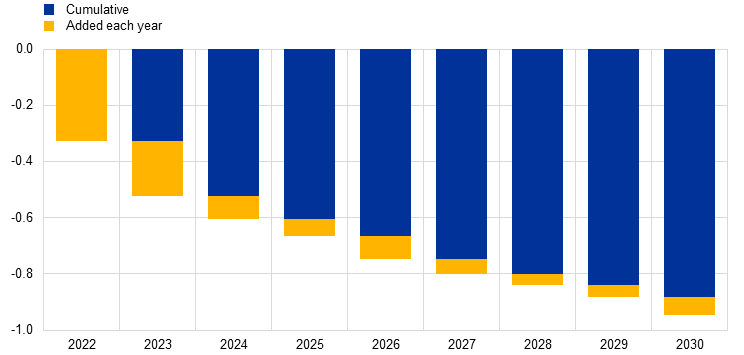
Sources: ECB (BSI, MIR, CES) and ECB calculations.
Notes: The chart illustrates the cumulative impact of increased mortgage payments on consumption under the assumption of no anticipation of consumption effects (myopia). For 2022 and 2023, changes in average consumption primarily reflect the influence of interest rate hikes on ARMs. Using the individual rate adjustments that originate in Chart 3, the new difference in year-on-year rates is multiplied by the depreciated outstanding balance (calculated by deducting principal payments over 12 months), and the resulting monthly payment change is subtracted from the previous year’s projected consumption. This adjustment is scaled by income-specific MPCs and an MPC of 1 for hand-to-mouth households. The aggregate consumption for each year is calculated, and the year-on-year change in mean consumption is derived. The latest data are for February 2025 for the CES mortgage stock, April 2025 for CES consumption and for January 2025 for MIR and BSI.
Box 2
The role of anticipation assumptions for the timing of consumption effects
Households are aware of changes in interest rates, especially in periods of significant monetary tightening.[11] They generally also know the structure of their mortgage and when it is set to reprice. Hence, forward-looking households exposed to interest rate risk could adjust their spending behaviour in anticipation of future rate changes. In this box we present evidence that these anticipation effects are limited and show how the timing of the impact on consumption varies under different assumptions.[12]
Chart A shows the consumption paths of different types of households with a mortgage over the past three years. First, we observe that households with a mortgage whose interest rate was set to change in 2024 (yellow line) started reducing consumption in the last quarter of 2023, and mostly reduced it going into 2024 – in contrast to mortgagors whose rate is not due to reprice in the next three years (blue line), who kept gradually increasing their consumption with no inflection point around 2024. Second, we observe that mortgagors whose mortgage is set to reprice between 2025 and 2027 (red line) have not yet shown any sign of reducing consumption and have behaved in a way more similar to the mortgagors whose rate is not set to reprice.
Chart A
Nominal consumption by group of mortgagors around a repricing year
(EUR)
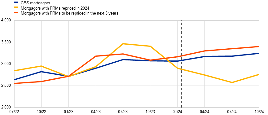
Sources: ECB (CES) and ECB calculations.
Notes: The chart depicts the backward consumption path of CES mortgagors, those with FRMs that were repriced in 2024, and those with FRMs set to be repriced in the next three years. Consumption in the CES is reported on a quarterly basis and respondents are asked about their expenditure on several items during the previous month. We aggregate these responses for each respondent and report two-quarter moving means.
In an effort to better evaluate the possible bounds of future effects on aggregate consumption, we construct two corner case scenarios – a no-anticipation scenario and a full anticipation scenario – as well as a more realistic one informed by the data: the partial anticipation scenario.
For the no-anticipation scenario, consumption effects are assumed to materialise only when mortgage payments increase (i.e. households are fully myopic or display no consumption-smoothing behaviour). The increased payments are then multiplied by income group-specific marginal propensities to consume (MPCs), which implies that only a percentage of the actual increase in costs is passed through to consumption. This is the scenario considered in the main text (Chart 4). We also assume a full pass-through for budget-constrained households.
Under the permanent income hypothesis and households’ preference for consumption smoothing, we can construct the other corner scenario, where households fully smooth out expected interest rate changes even if their lending rate is only due to change in the future. Assuming perfect foresight too, their interest rate expectation exactly matches that of the market. Only households that are budget-constrained to such a degree that they are unable to decrease consumption now are assumed to react only when their individual interest rate changes. For the rest, the accumulated consumption effects are broadly frontloaded to the periods when lending rates on new business adjusted (in 2022 and 2023), reflecting the timing of monetary tightening. The proportion of consumption adjustment in each of the two years is proportional to the size of interest rate increases that happened in each.
Finally, we also construct a more realistic scenario by estimating the timing and extent of anticipation effects. Leveraging our micro data, we compare the consumption of households with rates set to reprice in 2024 with the consumption of households whose rate is not set to reprice in the next three years. We identify few anticipation effects: the former only start reducing consumption relative to the latter in October 2023, i.e. with a lead of one quarter. Using a difference-in-differences approach, we estimate that only around 27% of the overall adjustment implied by the change in rates occurs in the year prior to it, with the remaining 73% happening in the year of the interest rate change (Chart B).
Chart B
Estimated impact on consumption of a mortgage rate reset in 2024
(EUR)
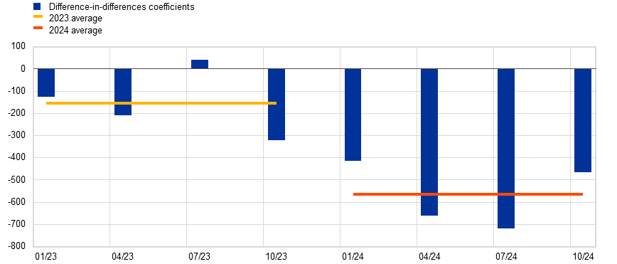
Sources: ECB (CES) and ECB calculations.
Notes: The chart depicts the coefficients from a difference-in-differences regression where we estimate the anticipation effect of increased mortgage payments of mortgagors with an FRM repriced in 2024. These results inform our partial anticipation scenario: by comparing the average effects of 2023 with those of 2024, we estimate the one-year-ahead anticipation effect to be approximately one-quarter of the total effect on consumption.
The latest observation is for October 2024.
Chart C illustrates the impact of increased mortgage payments on consumption under the three sets of assumptions. The solid bars reflect our main scenario holding rates on new loans constant at their latest level. The dashed bars show the pipeline effects if rates instead remain constant at their slightly higher end-2024 level. In the full anticipation scenario, the changes in consumption occurring in 2022-24 are around two-thirds of the total. However, about one-third of the total still takes place in 2025-30 due to the presence of (i) budget-constrained households that cannot adjust their consumption immediately, and (ii) new loans that, on average, start at higher interest rates than those that get fully repaid and drop out of the mortgage stock. These two factors imply that the pending consumption effects are still significant for the full anticipation scenario. In the more realistic partial anticipation scenario, 35% of the adjustment is yet to materialise by 2030.
Chart C
Impact on aggregate consumption growth under different anticipation assumptions
(cumulative percentage points)

Sources: ECB (BSI, MIR, CES) and ECB calculations.
Notes: The chart illustrates the cumulative impact of increased mortgage payments on consumption under three scenarios related to the anticipation of consumption effects: no anticipation (myopia), full anticipation (perfect foresight) and partial anticipation. The dashed bars show the conditional on December 2024 simulated results and the solid bars show the May 2025 update. For 2022 and 2023, changes in average consumption primarily reflect the influence of interest rate hikes on ARMs. Using the individual rate adjustments that originate in Chart 3, the new difference in year-on-year rates is multiplied by the depreciated outstanding balance (calculated by deducting principal payments over 12 months), and the resulting monthly payment change is subtracted from the previous year’s projected consumption. This adjustment is scaled by income-specific MPCs and an MPC of 1 for hand-to-mouth households. The aggregate consumption for each year is calculated, and the year-on-year change in mean consumption is derived.
The latest observations are for February 2025 for the CES and March 2025 for MIR and BSI.
Household income heterogeneity amplifies the effect of rate hikes early in the cycle. Poorer households have a higher share of mortgages due to reprice in the short term, as well as higher MPCs. These households are thus expected to be affected by rate hikes earlier on, with a disproportionate impact on consumption compared with a situation where MPCs are identical across households. Looking ahead, although lower-income households are expected to see a slower increase in their mortgage payments, they may still cut spending more due to this higher sensitivity. At the same time, households in the lower income quantiles hold lower shares of the aggregate stock of loans and represent a smaller share of total consumption, which should mitigate the role of MPC heterogeneity for the aggregate. In a scenario where MPCs are the same for all households, we find that the overall drag on consumption between 2022 and 2030 would be around 15% smaller. The further drag from heterogeneous MPCs persists throughout the entire period because lending rates on the stock of loans are expected to increase more for poorer households over that period.
The drag on consumption that has yet to materialise following the latest tightening cycle is large compared with previous cycles. The easing cycle that started in June 2024 led to a brief stabilisation of the rates paid by households on their stock of mortgages, which are expected to further increase starting in mid-2025. In contrast, and for reasons outlined above, when previous easing cycles began, the rates paid on outstanding balances declined. As detailed in Box 1, the remaining drag on consumption would be nil in our main scenario if the easing cycle had started with the rate configuration of October 2008.
5 Conclusion
In this article we explore how monetary policy affects consumption through changes in mortgage rates. Our simulations using household-level data show that, due to the higher prevalence of fixed-rate mortgages than in the past and the different configurations of interest rates on newly granted loans compared with outstanding loans, the cash flow channel is still expected to exert significant tightening pressure. Other things being equal, this should further dampen consumption through rising mortgage payments, despite the ongoing easing cycle. Our analysis underscores the importance of heterogeneity in monetary policy transmission by highlighting differences in mortgage contracts across countries and income groups. Poorer households tend to have more adjustable-rate mortgages or fixed-rate mortgages with shorter fixation periods, which means they are affected earlier in the cycle. In the current cycle, they will have been the ones experiencing the highest rise in interest payments by the end of 2030, with disproportionate effects on consumption due to their higher marginal propensities to consume.
Overall, the impact of monetary policy on consumption via the mortgage component of the cash flow channel is estimated to be significant. The impact on aggregate consumption amounts to 1 percentage point between 2022 and 2030, with 35% of the effects yet to materialise. However, it is important to note that this analysis focuses on one specific channel of adjustment and does not aim to provide a complete assessment of ongoing consumption developments, which also include positive effects from the recovery of real incomes and consumer confidence, in a context of monetary policy easing.
See, for example, Peersman, G. and Smets, F., “The monetary transmission mechanism in the euro area: evidence from VAR analysis”, in Angeloni, I., Kashyap, A.K. and Mojon, B. (eds.), Monetary Policy Transmission in the Euro Area, Cambridge University Press, Cambridge, 2003.
Auclert, A., “Monetary Policy and the Redistribution Channel”, American Economic Review, Vol. 109, No 6, 2019, pp. 2333-67.
Di Maggio, M., Kermani, A., Keys, B.J., Piskorski, T., Ramcharan, R., Seru, A. and Yao, V., “Interest Rate Pass-Through: Mortgage Rates, Household Consumption, and Voluntary Deleveraging,” American Economic Review, Vol. 107, No 11, 2017, pp. 3550-88; Floden, M., Kilstrom, M., Sigurdsson, J. and Vestman, R., “Household Debt and Monetary Policy: Revealing the Cash-Flow Channel”, Swedish House of Finance Research Paper, No 16-8, 2017; Kaplan, G., Moll, B. and Violante, G.L., “Monetary Policy According to HANK”, American Economic Review, Vol. 108, No 3, 2018, pp. 697-743; and Slacalek, J., Tristani, O. and Violante, G.L., “Household balance sheet channels of monetary policy: A back of the envelope calculation for the euro area”, Journal of Economic Dynamics and Control, Vol. 115, 2020.
See, for example, the boxes entitled “What explains the high household saving rate in the euro area?”, Economic Bulletin, Issue 8, ECB, 2024, and “Are real incomes increasing or not? Household perceptions and their role for consumption”, Economic Bulletin, Issue 1, ECB, 2025.
All numbers reported are weighted by population weights and the size of the loan.
See Lusardi, A. and Mitchell, O., “The Economic Importance of Financial Literacy: Theory and Evidence”, Journal of Economic Literature, Vol. 52, 2014, pp. 5-44.
This summary statistic is also put forward as relevant for the refinancing channel of monetary policy in Eichenbaum, M., Rebelo, S. and Wong, A., “State-dependent effects of monetary policy: The refinancing channel”, American Economic Review, Vol. 112, No 3, 2022, pp. 721-761.
All rates on fixed-rate loans are then adjusted by the same amount to match the aggregate October 2008 rate on outstanding amounts.
Budget-constrained households are defined as those with housing and food expenses above 75% of their total household income.
MPCs are estimated by combining the income elasticity of consumption with the mean average propensity to consume (APC) per income quintile. The income elasticity is estimated for the complete sample based on quarterly data on nominal consumption and annual data on household income. The APC is calculated by combining the consumption and income data and aggregating by income quintile. These estimates refer to transitory shocks and are somewhat higher than – but broadly in line with – Ampudia, M., Cooper, R., Le Blanc, J. and Zhu, G., “MPC Heterogeneity and the Dynamic Response of Consumption to Monetary Policy”, American Economic Journal: Macroeconomics, Vol. 16, No 3, 2024, pp. 343-388. However, they are lower than MPCs of permanent shocks, which are closer to 1. For a comprehensive review of the literature on MPC, see also Kaplan, G. and Violante, G.L., “The marginal propensity to consume in heterogeneous agent models”, Annual Review of Economics, Vol. 14, 2022, pp. 747-775.
See, for example, Charalambakis, E., Kouvavas O. and Neves, P., “Rate hikes: How financial knowledge affects people’s reactions”, The ECB Blog, ECB, 15 August 2024.
This is consistent with the literature rejecting the permanent income hypothesis. See, for instance, Johnson, S.D., Parker, A.J. and Souleles, N.S., “Household Expenditure and the Income Tax Rebates of 2001”, American Economic Review, Vol. 96, No 5, 2006, pp. 1589-1610.